A split-core current transformer makes it easy to measure current without cutting wires.
The core of a split-type current transformer can be opened, allowing wires to be threaded through the center and secured. This transformer is suitable for applications where cutting wires is not possible. The video demonstrates how to connect and test a current transformer, monitor output current and voltage, and use a rectifier to convert AC to DC.
Split-core current transformers provide excellent isolation and ease of use for power measurement.

What is the difference between an autotransformer and an isolation transformer?

Autotransformer:

An autotransformer is a transformer whose windings are primary and secondary on the same winding. According to the structure, it can also be divided into adjustable voltage type and fixed type. The coupling of autotransformer means electromagnetic coupling. Ordinary transformers transfer energy through electromagnetic coupling of primary and secondary coils. There is no direct electrical connection between the primary and secondary sides. The primary and secondary sides of autotransformers have direct electrical connection, and its low-voltage coil is part of the high-voltage coil. Autotransformers and other protective equipment are also used in the protection equipment of communication lines.

An autotransformer is a self-coupling transformer. The autotransformer structure is relatively simple, low cost, and the input/output and neutral line are shared. The secondary side of the transformer is part of the primary side. The primary and secondary sides share a winding, like two coils coming out of a line. The two coils use the difference of the current to cut the magnetic lines of force to transform the voltage. It is generally used in the boost of DC power. The output and input of the transformer have direct electrical connection, and the safety performance is poor.

Isolation transformer:

Isolation transformer refers to a transformer with electrical isolation between the input winding and the output winding. Isolation transformer is used to avoid accidental contact with live objects at the same time. The isolation of the transformer is to isolate the current of the primary and secondary windings. It was used in the power industry in European countries in the early days, and is widely used in the control power supply of general circuits in the electronics industry or industrial and mining enterprises, machine tools and mechanical equipment, and the power supply of safety lighting and indicator lights.

The main function of the isolation transformer is to isolate the electrical equipment from the power grid. It is used in safety occasions or occasions with anti-interference requirements. There is no direct electrical connection between the electrical equipment and the power supply. The isolation structure has many materials and high cost. In addition to changing the voltage, it can also electrically isolate the input winding and the output winding from each other, and isolate the input/output and the neutral line to avoid the danger of touching the live object (or metal parts that may be charged due to insulation damage) and the ground at the same time. In addition, the isolation transformer also has a certain effect of suppressing various interferences, has filtering performance, and is highly safe.

The difference between autotransformer and isolation transformer:

1. Difference in structure

Isolation transformer is the most common transformer. Its low-voltage and high-voltage windings are wound by separate coils and have no electrical connection. There is no direct electrical connection between the primary and secondary sides, and the secondary winding is not connected to the ground.

The primary and secondary sides of the autotransformer have direct electrical connection. Its low-voltage coil is part of the high-voltage coil, that is, a winding with only one electrical path. There is a tap in the middle of the winding as the common point of the high-voltage and low-voltage coils.

2. Difference in safety factor

Usually, one line of the AC power supply voltage we use is connected to the ground, and the other line has a potential difference of 220V or 380V with the ground. People will get electric shock if they touch it. The secondary high and low voltage coils of the isolation transformer are electrically insulated from each other and are not connected to the ground. There is no potential difference between any two of its lines and the ground. People will not get electric shock if they touch any line, which is safer. Therefore, no matter whether the secondary voltage exceeds the safe voltage value, as long as the person does not touch the two output points of the secondary with voltage difference at the same time, it will not cause harm to people. This is the biggest advantage of the isolation transformer. But it is large in size and high in cost.

Because the high and low voltage coils of the autotransformer overlap, some coil wire materials are saved, which is not only small in size but also low in cost. However, its high and low voltage coils are connected. Even if the output voltage of the low voltage side of the step-down transformer is very low, because its two windings have a common part, the primary high voltage will “sneak into” the secondary coil, which is very easy to cause harm to people.

3. Differences in use

Three-phase isolation transformers are mainly used for power loads of power systems and industrial and mining enterprises, and power sources that require isolation from the power grid to convert the mains electricity into magnetic electricity. They are used as power equipment for precision measurement and test purification (anti-interference) of power and power grid. Isolation transformers are safe power supplies and are generally used for machine maintenance to protect, prevent lightning, and filter.

The primary and secondary sides of the autotransformer are directly connected electrically. If the line is damaged or leaking, it is very easy to cause harm to people. It is generally used in places where safety requirements are not high. It only needs to change the voltage so that the voltage meets the required voltage of the equipment. However, the equipment cannot be equipped with a leakage protection device and the neutral wire cannot be grounded.

The difference between switching power supply and linear power supply: comprehensive analysis and comparison

 
In the huge system of electronic equipment, the power supply is a key part to ensure the stable operation of the equipment. As two common types of power supplies, switching power supply and linear power supply have obvious differences in multiple dimensions, which directly affect the applicability of power supply in different scenarios. Understanding their differences is very important for professional electronic engineers to design circuits or ordinary electronic enthusiasts to maintain and use electronic equipment.

Ⅰ. Working principle: different energy conversion methods

1. Switching power supply: high-frequency switching

The core of the switching power supply is that the switch tube is turned on and off at high frequency. Take the common Buck step-down circuit as an example:

Conduction phase: When the switch tube is turned on, the input voltage is loaded on the inductor, the inductor begins to store energy, and the current supplies power to the load and charges the output capacitor at the same time, and the inductor current gradually increases.
Turn-off phase: When the switch tube is turned off, the current in the inductor cannot change suddenly, so it will form a loop through the freewheeling diode, continue to supply power to the load, and the inductor current gradually decreases.
Control method: The output voltage is precisely controlled by adjusting the proportion of the switch tube conduction time in the entire switching cycle (i.e., the duty cycle).

For example, converting a 12V input to a 5V output is achieved by adjusting the duty cycle. The operating frequency of the switching power supply is usually between tens of kHz and several MHz. The high-frequency operating characteristics enable it to use miniaturized inductors, capacitors and other energy storage components to effectively improve the power density.

2. Linear power supply: Continuous voltage regulation of linear components

Linear power supplies use the linear amplification characteristics of linear adjustment components (such as Linear Transformer) to stabilize the output voltage:

Basic process: The input AC power is first stepped down by the transformer, and then converted to DC power by the rectifier. After preliminary smoothing by the filter capacitor, the linear adjustment tube continuously adjusts the internal resistance according to the feedback signal to stabilize the output voltage.

Working state: The linear adjustment tube always works in the linear amplification area, and the current passes continuously, ensuring the stability of the voltage adjustment process.

This continuous adjustment method makes the output voltage more stable and is suitable for scenarios with high voltage accuracy requirements.

Ⅱ. Efficiency performance: the difference between high and low is obvious

1. Switching power supply: high efficiency and energy saving

The efficiency of switching power supply is usually between 70% and 95%, mainly due to the following characteristics:

When turned on: the internal resistance of the switch tube is extremely small, and the heat loss is low when the current passes through.

When turned off: almost no current passes, and the power loss can be ignored.

Only at the moment of switching: a certain loss is generated due to the overlap of voltage and current, but the overall proportion is small.

In high-power applications (such as server power supplies and industrial equipment), the high efficiency characteristics of switching power supplies can significantly reduce energy consumption and save operating costs.

2. Linear power supply: relatively low efficiency

The efficiency of linear power supply is generally between 30% and 60%, mainly because:

The linear adjustment tube needs to continuously consume its own power to adjust the output voltage.

When the input and output voltage difference is large, the power loss on the adjustment tube is significant, and a large amount of electrical energy is wasted in the form of heat energy.

For example, when the input is 12V and the output is 5V, the adjustment tube needs to bear a 7V voltage drop, and this part of the energy is all converted into heat. Therefore, linear power supplies are mostly used in low-power and low-efficiency applications.

III. Output ripple characteristics: significant differences in size

1. Switching power supply: relatively large ripple

Due to its pulsed working mode, the output ripple of the switching power supply is large. Although the ripple can be reduced by adding a filter circuit (such as electrolytic capacitor + ceramic capacitor in parallel), its ripple level is still higher than that of the linear power supply.

Applicable scenarios: Applicable to equipment with low ripple requirements, such as ordinary motor drive power supplies.

Restricted scenarios: Not applicable to circuits with high requirements for power purity, such as precision analog signal processing or high-end audio equipment.

2. Linear power supply: small ripple

Linear power supply has extremely small output ripple through linear adjustment and smooth filtering, and is suitable for:

High-precision measurement equipment (such as oscilloscopes, medical diagnostic instruments)
Systems with extremely high voltage stability requirements (such as scientific research instruments, precision amplifier circuits)

IV. Volume and weight: obvious differences

1. Switching power supply: small and light

Switching power supply has a high operating frequency, can use small inductors and capacitors, and does not require large power frequency transformers, so:

Small size and light weight

High power density: can provide higher power at the same volume

Widely used in portable devices (such as mobile phone chargers, tablet power adapters) and systems with strict space requirements.

2. Linear power supply: large size and weight

Linear power supply has a low operating frequency, and requires the use of large-size power transformers and large-capacity filter capacitors, resulting in:

Large size and heavy weight

Not suitable for space-constrained equipment

In occasions such as portable medical equipment and small drones, linear power supplies may be limited by volume issues

Ⅴ. Response speed: different speeds

1. Switching power supply: relatively slow response

Due to the presence of energy storage components such as inductors and capacitors, it takes a certain amount of time to adjust the output voltage when the load changes suddenly. Although the response speed can be improved by optimizing the control circuit, the response speed improvement is limited by the characteristics of the energy storage components.

Applicable scenarios: equipment with infrequent load changes

2. Linear power supply: fast response

The linear power supply adjustment tube can quickly adjust the internal resistance and respond to load changes. It is suitable for:

Audio amplifier (need to quickly follow the audio signal)

High-speed data acquisition system

Precision motion control system

Ⅵ. Electromagnetic interference characteristics: different strengths

1. Switching power supply: strong electromagnetic interference

Switching power supply will generate high-frequency harmonics during high-frequency on/off, resulting in strong electromagnetic interference (EMI):

Conducted interference: conducted through the power line

Radiated interference: radiated through space

To reduce interference, filtering, shielding, and optimized PCB layout measures are required, which increase the design complexity and cost.

2. Linear power supply: weak electromagnetic interference

Linear power supply has low operating frequency, and the main sources of electromagnetic interference are transformer leakage and rectifier noise. The interference frequency is low and the intensity is weak, so almost no additional suppression measures are required.

Applicable scenarios: Environments that are sensitive to electromagnetic interference, such as near wireless communication equipment

The SCT013 series are sensors of non-invasive, current transformers that measure the intensity of a current that crosses a conductor without needing to cut or modify the conductor itself.  We can use these sensors with a processor, like Arduino, to measure the intensity or power consumed by a load.

The SCT013 sensors are current transformers, instrumentation devices that provide a measurement proportional to the intensity that a circuit crosses. The measurement is made by electromagnetic induction.

SCT013 sensors have a split core (like a clamp) that allows the user to turn it on to wrap electrical equipment without having to cut it off.

In the SCT013 series there are models that provide the measurement as a current or a voltage output. It is more preferable to use voltage output because the connection is simpler.

The sensor accuracy can be off by only 1-2%. To ensure highest accuracy, it is critical to confirm that the core has been properly closed. Even a small air gap can cause a 10% deviation.

As a disadvantage, being an inductive load, the SCT013 introduces a variation of the phase angle, whose value is a function of the load that passes through it, being that it is able to reach up to 3º.

Current transformers are common components in the industrial world as well as in electrical distribution, as they allow the points of consumption to be monitored, whereas another form of measurement does not exist. They are also considered multiple measurement instruments, even in portable equipment such as perimeter clamps or network analyzers.

For example, in our electronics and home automation projects, we can use the SCT013 current sensors to measure the electrical consumption of a device, check the status of an electrical installation, and to record the consumption of electricity in home energy monitors. an installation or even access through the internet in real time.

PRICE

The SCT013 series has a variety of models that can change the measurement range and output shape. Physically, they are the same, although it is possible to identify them by the text written on the product shell.

The price of all models is similar, and we are looking for international sellers such as eBay, Amazon or AliExpress.

The most common model is SCT013-000, of which the maximum current is 100A, the current output is 50mA (100A:50mA), the maximum current of SCT-013-030 is 30A (30A/1V), and the voltage output is 1V.

Finally, while it is important to have a wide range of measurements, it is important to bear in mind that a higher intensity model will result in less precision. An intensity of 30A to 230V corresponds to a load of 6,900W, which is enough for most home users.

How does the SCT013 work?

The SCT013 sensors are small current transformers, or CTs. Current transformers are instruments widely used for measuring elements.

A current transformer is similar to a voltage transformer and is based on the same operating principles (in fact, they were previously identical). However, they have different objectives and, as a result, are designed and constructed differently.

A current transformer seeks to generate an intensity in the secondary that is proportional to the intensity that passes through the primary. For this, it is desired that the primary is formed by a reduced number of turns.

We can use the current transformer to build non-intrusive current sensors. In the current sensor, the ferromagnetic core can be separated so that the conductor can be opened and rolled up.

So, we have a transformer, it is:

• The cable through which the current to be measured is the primary winding
• The “clamp” is the magnetic core.
• The secondary winding is integrated as part of the probe.

When the alternating current circulates through the conductor, a magnetic flux is generated in the ferromagnetic core, which in turn generates an electrical current in the secondary winding.

The intensity transformation ratio depends on the relationship between the number of turns:

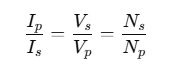
The primary is usually formed by a single loop made by the conductor to be measured. Although, it is possible to wind the driver making this happen more than once inside the “clamp”. The number of turns of the secondary, integrated in the probe, varies from 1000-2000, according to the models of the SCT013.

Unlike voltage transformers, in a current transformer, the secondary circuit should never be opened, because induced currents could damage the component. For this reason, the sensors of SCT13 have protections: resistance burden in the sensors of output by voltage, or diodes of protection in the sensors of exit by the current.

Assembly Diagrams

To understand the connection of the sensor SCT013, we have to understand and solve three problems:

 Sensor output in intensity

 Adjustment of the voltage range

 Positive and negative stress

SENSOR OUTPUT IN INTENSITY

The SCT013 are current transformers, that is, the measurement is obtained as an intensity signal proportional to the current flowing through the cable,.  Processors, however, are only capable of measuring voltages.

This problem is easy to solve. To convert the output in intensity into a voltage output, we only have to include a resistance (load resistance).

With the exception of model SCT013-000, all other SCT013 models have an internal load resistance so that the output is a voltage signal of 1V. This is why it will not be a concern to worry about.

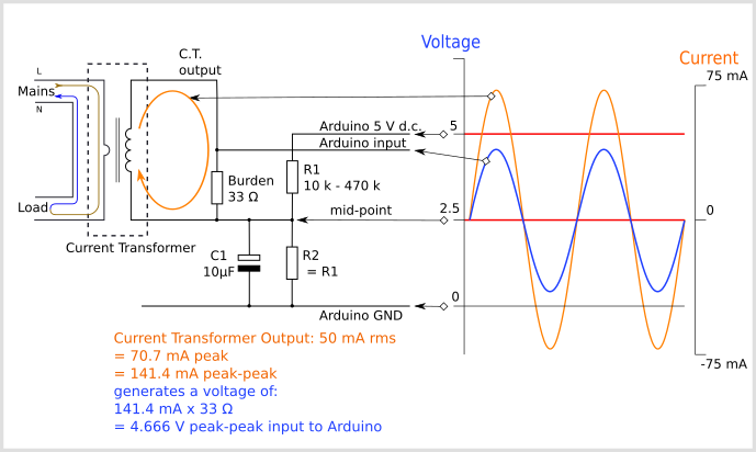
Only in the case of SCT013-000, there is no resistance internal burden, so the output is a signal of ± 50mA. A resistance of 33Ω in parallel with the sensor will suffice.

Positive and Negative Tensions

Another problem we have to solve is that we are measuring alternating current, and the intensity induced in the secondary is alternating. After passing through the resistance burden, whether internal or external, the voltage output is also alternating.

However, as we know, the analog inputs of the majority of processed currents, including Arduino, can only measure positive voltages.

To measure the voltage at the transformer output, we have several options, ordered here from least to most recommended:

1. Rectify the signal through a diode bridge, and measure the wave as positive values. Not advisable given that we lose information as to whether we are in the negative or positive half-period, and because we will have the voltage drop of the diode, and, even worse, the diode does not drive below a voltage meaning the signal will be distorted at the junctions by zero.
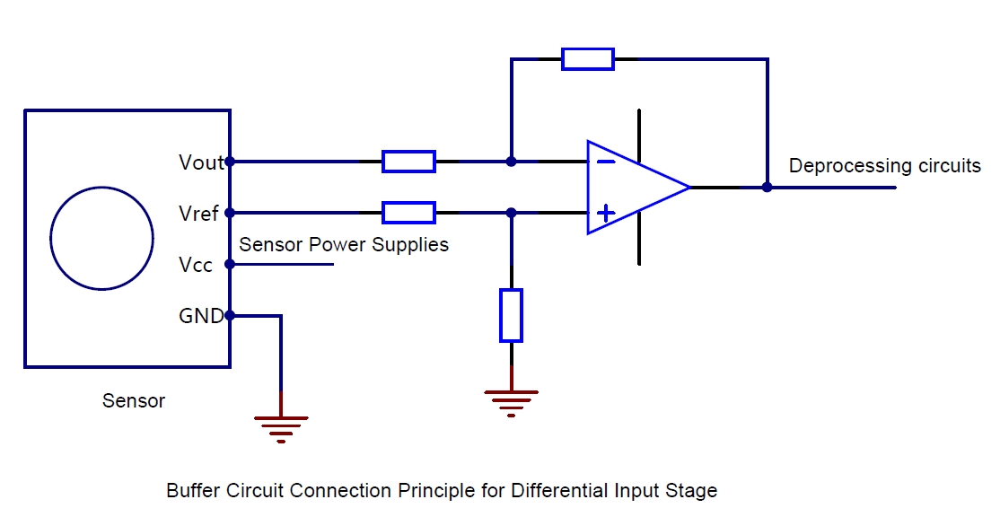
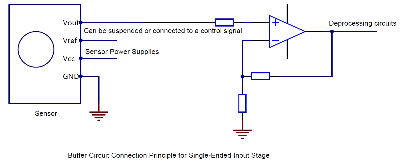
2. Add an offset in DC by using two resistors and a capacitor that provide a midpoint between GND and Vcc. Much better if we also add an operational amplifier as a voltage follower.
3. Add an ADC with differential input, which allows measurements of positive and negative voltages, such as the ADS1115. This is the option that we are going to use.

Voltage Range Adaptation

The last problem is the need to adapt the range of voltages at the sensor output. Arduino can only perform measurements between 0 and Vcc. In addition, the smaller the range, the greater loss of accuracy, so we should adapt to this range.

On the other hand, we must remember that when it comes to AC voltage, RMS values are usually used. Briefly review the peak voltage and peak-to-peak equations:

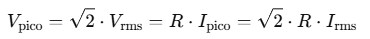
Therefore, for a sensor with an output of ±1V RMS, the peak voltage is ±1.414V and the

In the case of the SCT013-000, the output will be ±50mA. With an external load resistance of 33Ω, the output voltage is ±1.65V RMS, so the peak voltage is ±2.33V and the peak-to-peak voltage is 4.66V.

Electric Connection

We already have all the components to measure the network intensity with an SCT-013 sensor. We will use a sensor with voltage output ± 1V RMS and internal burden resistance, together, with an ADC like the ADS1115 in differential mode.

Adjusting the gain of the ADS1115 to 2.048V will place it within the range of ± 1.414V. In the case of a 30A sensor we will have an accuracy of 1.87mA, and 6.25 mA for a 100A sensor.

If you use an SCT013-000 with an output of ± 50mA, we will have to add an external load resistor of 33Ω and raise the gain of the ADS1115 to 4.096V to comply with the range of ± 2.33

The connection, seen from Arduino, would only be the power supply of the ADS1115 module as we saw in the entry on the ADS1115.

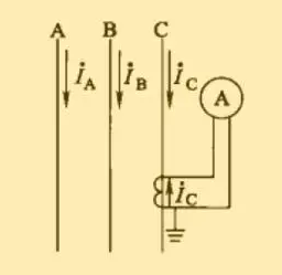
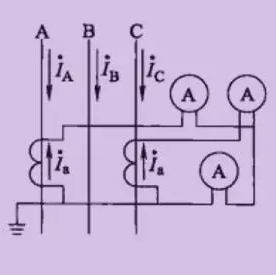
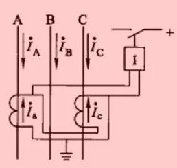
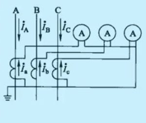
For the measurement, it is important that we use only one wire in the “clamp” If we use multiple conductors (two conductors for a single-phase installation and three for a three-phase installation), the role of the conductor will be abolished. This produces a zero inductance, and therefore produces an empty measurement.

The SCT013 sensor has a Jack 3.5 connector, which is very common in the audio field but is not sufficient to use in our electronic projects. To be able to connect it, we must cut off the cable or get a female connector off our welding cable. Fortunately, these terminals are easy to get, but do not rule out cutting off the cables.

If you don’t want to use an external ADC, you can also use a more traditional solution that adds a circuit that allows us to add a center offset.

From now on, we will assume that you use an Arduino with Vcc 5V. If you use another processor or an Arduino model with another Vcc (for example, 3.3V), you should correct the part accordingly.

When we added a 2.5V DC offset point, the final range was 1.08V to 3.92V, with Arduino powered at 5V over the analog input range.

Code example.

Assembly with ADS1115

If you use a component with SCT013 with ±1V RMS output and ADS1115, the required code is similar to the code we see in the input to the ADS1115. You need to consult the Adafruit library for ADS1115.

In order to sample the ADS1115 at a higher speed, we need to modify the file, ‘Adafruit_ADS1015.h’.

With this modification, we will be able to reduce the sampling time from about 8-9 milliseconds (about 100 hertz) to about 1.8 milliseconds (about 500 hertz). As we leave the Nyquist frequency, we improve the measurement behavior.

Another version uses the measured maximum and minimum values and then calculates the measured value based on the peak value. The result should be similar to that seen in the square sum example. To do this, you can replace this feature with the following features:

We can see the results in the serial port monitor, and either draw them with a serial plotter, collect it in a larger project to display on a web page, or register it in SD.

ASSEMBLY WITH RESISTANCE AND MEDIUM POINT

In this case, the example is very simple and we only need to measure through analog input:

Why Use a Rogowski Coil?

Overview

Rogowski coils are specialized devices for measuring alternating current (AC) or high-speed current pulses, offering unique advantages for various applications. They are particularly useful in scenarios where flexibility, accuracy, and safety are crucial.

Flexibility and Ease of Use

Rogowski coils are flexible and can be wrapped around live conductors without disconnection, making them perfect for tight spaces or crowded electrical panels. This non-invasive installation reduces downtime and simplifies setup, especially in industrial or commercial settings.

High Current and Frequency Capability

Unlike traditional current transformers, Rogowski coils use an air core, preventing magnetic saturation. This allows them to accurately measure very high currents, such as those in power transmission or welding, and handle rapid changes, like transients or pulses, making them suitable for high-frequency applications.

Safety and Cost-Effectiveness

They are safer because they don’t produce high voltages when open-circuited, reducing electric shock risks. Additionally, their lightweight and simple design lowers construction and installation costs, offering a cost-effective solution for current measurement.

What is the Rogowski coil?

A Rogowski coil is a specialized electrical device designed for measuring alternating current (AC). It consists of a helical coil of wire wound uniformly around a non-magnetic, air-filled core, typically arranged in a toroidal (doughnut-like) shape. The coil is placed around a current-carrying conductor, and as the AC flows through the conductor, it generates a changing magnetic field. This changing magnetic field induces a voltage in the Rogowski coil, which is proportional to the rate of change of the current (the time derivative, di/dt).

To obtain a direct measurement of the current, the induced voltage is typically processed through an integrator circuit, which converts the voltage signal into one proportional to the current itself. This makes the Rogowski coil particularly useful for applications requiring the measurement of high currents or fast transient currents, such as in power systems, industrial equipment, or research settings.

Key Features and Advantages

Air Core Design: Unlike traditional current transformers with iron cores, the Rogowski coil’s air core prevents magnetic saturation, allowing it to measure very high currents without distortion.
Flexibility: Many Rogowski coils are designed to be flexible and can be opened to wrap around a conductor without needing to disconnect it, making installation straightforward and non-invasive.
Wide Bandwidth: The coil can accurately measure currents with high-frequency components or rapid changes, such as those in lightning strikes or switching transients.

Applications

Power system monitoring and protection.
Measuring high currents in welding or industrial processes.
Research applications, such as analyzing transient phenomena.

Understanding Current Transformers and Their Applications

Current transformers (CTs) are essential components in modern electrical systems. They allow for the safe measurement, monitoring, and control of high currents by producing a scaled‐down replica of the current flowing in a conductor. This article delves into how current transformers work, their various types, and the diverse applications in which they are used.

What Are Current Transformers?

Current transformers are devices designed to measure high electrical currents by generating a lower, proportional current that can be easily and safely measured by standard instruments. They serve as a bridge between high-power circuits and sensitive electronic equipment, ensuring that monitoring and control systems can operate without being exposed to dangerous high currents.

How Do Current Transformers Work?

At their core, current transformers work on the principle of electromagnetic induction. When a current flows through the primary conductor (which can be as simple as a single wire passing through the CT’s core), it produces a magnetic field. This magnetic field induces a current in the CT’s secondary winding. The ratio of the number of turns in the primary winding (often just the conductor itself) to the number of turns in the secondary winding determines the scale factor, which in turn sets the output current relative to the primary current.

For example, a CT designed to provide a 1 A secondary output might have a ratio of 3000:1, meaning that when 3000 A flows in the primary circuit, the CT outputs 1 A. In many cases, the secondary output is standardized (such as 1 A, 5 A, or even a voltage output like 0.333 V) to simplify instrumentation and protection system designs.

Types of Current Transformers

There are several types of current transformers available, each suited to different applications:

• Solid-Core (or Wound-Core) CTs:
  These are built with a fixed, solid magnetic core. They are typically used in new installations where the CT can be designed and manufactured as an integral part of the system.
• Split-Core (or Open-Core) CTs:
  These CTs are designed with a hinge or split mechanism, allowing them to be clamped around an existing conductor without the need to disconnect it. This makes them ideal for retrofitting into operational systems and for applications where safety and ease of installation are paramount.
• Bar-Type CTs:
  In these models, the CT is integrated directly into busbars or conductors, offering robust performance in high-current scenarios.
• Rogowski Coils:
  Although technically not transformers in the traditional sense, Rogowski coils are used to measure alternating currents. They offer the advantage of being flexible and non-intrusive but require integrator circuits to produce a voltage output proportional to the current.

Key Applications of Current Transformers

Current transformers have a wide range of applications across various sectors:

1. Energy Metering

CTs are fundamental in electricity metering, allowing utilities and consumers to accurately measure energy consumption. By stepping down the high currents found in power distribution systems to measurable levels, CTs enable precise billing and energy monitoring.

2. Protection Systems

In protection relays and circuit breaker control, CTs provide crucial information about the current flowing through a circuit. This data helps in detecting abnormal conditions, such as overloads or short circuits, and initiates protective measures to isolate and protect equipment.

3. Control and Monitoring

Industrial automation and control systems use CTs to monitor current levels in motors, transformers, and other equipment. This monitoring helps in managing system performance and efficiency while ensuring that components operate within safe parameters.

4. Renewable Energy Systems

In renewable energy installations, such as wind farms and solar power plants, CTs are used to monitor the flow of electricity from generation to the grid. They ensure that systems operate efficiently and safely while providing data for performance optimization.

5. Safety and Instrumentation

CTs help in ensuring personnel safety by enabling the use of isolated measurement instruments. By providing a low-level secondary current, CTs allow for the safe operation of meters and sensors that would otherwise be at risk if connected directly to high-current circuits.

Used to characterize dynamic behavior of a transducer, step response time is the delay between the primary current reaching 90% of its final value and the transducer’s output reaching 90% of its final amplitude. The primary current shall behave as a current step, with a given di/dt slope (usually 100A/µs) and with the amplitude close to the nominal current value I_PN .

The residual magnetic flux (remanence) of the core varies depending on the sensor type and the magnetic material and causes an additional measurement offset, called “magnetic offset”. The value of the magnetic offset depends on the previous magnetization of the core and reaches a maximum value after the magnetic circuit is saturated.

Magnetization can occur in the following situations:

1. High overload current

2. Power supply interruption (power failure)

The offset caused by magnetization disappears in the following situations:

1. The offset caused by magnetization disappears naturally (the core recovers slowly, the speed depends on the magnetic material)

2. It is eliminated by demagnetizing the sensor, for example by appropriately reversing the primary current or using a dedicated demagnetization cycle. After demagnetization, the sensor can restore its initial performance.

Process of Demagnetization:

To demagnetize a transducer’s magnetic core, the following steps are typically used:

1.AC Excitation: A low-frequency AC source drives the magnetic core through its entire B-H hysteresis loop (the magnetic field vs. magnetization curve), applying alternating current to cycle the core’s magnetization from positive to negative saturation.

2.Gradual Decrease of Excitation: After cycling the core through the B-H loop for at least 5 full cycles at maximum amplitude, the amplitude of the AC excitation is reduced gradually. The rate of reduction should be no faster than 4% per cycle to ensure a smooth return of the core’s magnetization to zero (the origin of the B-H curve).

3.Time Requirements: Typically, a demagnetization cycle will require around 30 cycles at a low frequency, such as 500 milliseconds at 60 Hz.

Special Considerations for Closed-Loop Devices:

For closed-loop transducers (devices that have a compensation coil), additional care is needed because the compensation coil can interfere with the demagnetization process by negating its effects. This interference can prevent the core from reaching its neutral state. Therefore, extra steps may be required to ensure proper demagnetization.

Partial Demagnetization:

Alternatively, partial demagnetization can be achieved by applying a specific signal of opposite polarity to the core’s magnetization. However, this method is more complex because it requires precisely determining the correct amplitude and duration of the signal to effectively reduce the magnetization without overshooting or undercompensating.

In practice, if a specific application is well understood, it is possible to determine the necessary correction signal empirically and apply this whenever demagnetization is needed.

Demagnetization is essential for maintaining the accuracy and reliability of a transducer’s measurements, especially after strong magnetic influences or long-term use.

Let’s take a product with a supply voltage of +5V and an output of 2.5V ± 0.625V with a precision of 1% as an example.
Our Vref pin serves two functions: one is to act as a reference point for output, commonly used in differential input acquisition devices; the other function is for single-ended input acquisition devices, where it is used to control the sensor output, making the static output (2.5V) more accurate. It only affects the static output (2.5V when there is auxiliary power and no input signal) and does not affect the amplification (0.625V).
Due to the discreteness of product parameters, sensors cannot be perfectly identical and ideal, and there will always be some degree of error. For most of our products, the static reference point error is within ±15mV. This means the static output of 2.5V (with 0V or GND as the reference point) will be between 2.485V and 2.515V, which is considered within the acceptable range.
For example, for a product with a power supply of +5V and an output of 2.5V ± 0.625V with a precision of 1%:

If the output is referenced to 0V (GND), we calibrate it as follows:
First, check if the Vref voltage meets the requirements (standard is 2.5V ± 1%, generally no more than 0.5%).
The second step is to adjust the static output to between 2.485V and 2.515V (i.e., 2.5V ± 15mV).
The third step is to apply the input signal to the rated input and adjust the output to within 2.5V + (0.625V ± 1%).
Finally, check if the output at 10% of the rated input is accurate. If there is significant error, adjust the zero-point component for correction. Then, check if the zero-point and full-scale values meet the requirements. If everything is correct, the product moves on to the next process step.

If the output is referenced to Vref, we adjust it as follows:

First, check if the Vref voltage meets the requirements (standard is 2.5V ± 1%, generally no more than 0.5%).
The second step is to adjust the static output to between 2.485V and 2.515V (i.e., 2.5V ± 15mV).
The third step is to connect the black probe of the multimeter to the Vref point, apply the input signal to the rated input, and adjust the output to within 0.625V ± 1%.
Finally, check if the output at 10% of the rated input is accurate. If there is significant error, adjust the zero-point component for correction. Then, check if the zero-point and full-scale values meet the requirements. If everything is correct, the product moves on to the next process step.

If a product adjusted using the first method is used in a differential input acquisition device, the acquired signal will be inaccurate and may even produce negative output errors.
If a product adjusted using the second method is used in a single-ended input acquisition device, the acquired signal will also be incorrect and may result in overflow errors.

By default, our products are calibrated using the first method (referenced to 0V/GND), as most customers request this.

Example 1: A product calibrated using the first method, with Vref = 2.510V and Vout = 2.505V in the static state. This product is qualified, and the precision is acceptable. However, when used in a differential input acquisition device, since Vout is lower than Vref, the static output will be negative, which is incorrect.

Example 2: A product calibrated using the second method, with Vref = 2.510V and Vout = 2.520V in the static state. This product is also qualified, as the zero-point error does not exceed 15mV. However, when used in a single-ended input acquisition device, the output of 2.520V exceeds the calibrated 15mV error, and the full-scale value will also be higher, which could reach up to 2% in extreme cases, affecting the customer’s use.
Now that some customers have reported this type of error, we are asking them to provide calibration requirements to correct the issue. Sales representatives are also being asked to label products based on different calibration methods to ensure correct production for customers.

In a current transformer (CT), the burden refers to the total impedance (resistance and reactance) presented by the connected measuring devices, such as ammeters, relays, or meters, to the secondary winding of the CT. It is usually expressed in volt-amperes (VA) at a specific secondary current (typically 1A or 5A) and can include the impedance of the connecting wires and instruments.

Key Points:

1. Burden Components: The burden consists of the impedance of the connected devices (like meters, protection relays, and wires) which draw power from the CT’s secondary winding.
2. Burden Rating:
   • CTs are rated for a maximum burden in VA. For example, a CT rated for 10 VA means that the connected load should not exceed 10 VA.
   • If the burden exceeds the CT’s rated value, it can cause errors in current measurement or protection malfunctions because the CT may not be able to maintain its accuracy or properly step down the current.
3. Importance of Proper Burden:
   • The burden affects the accuracy of the CT. If the burden is too high (i.e., the impedance of the connected devices is too large), the CT will not provide an accurate current transformation, leading to incorrect measurements or protection relay malfunctions.
   • On the other hand, if the burden is too low, the CT may operate closer to saturation, which also leads to inaccuracies.
4. Practical Consideration:
   • When installing a CT, it is crucial to calculate the burden of all connected devices and ensure it falls within the CT’s rated burden for proper performance.

In summary, the burden is the load imposed on the secondary winding of the current transformer, and ensuring it is within the CT’s rated capacity is essential for accurate current measurement and safe operation.

1. Single-Phase Circuit:

• Connection Mode: A single current transformer is connected in series with the live wire or neutral wire of the circuit.
• Application: This is used for measuring single-phase current, power, and providing protection against single-phase faults, such as ground faults or short circuits.
• Diagram:
• 

2. Incomplete Star (V Connection) for Two Current Transformers (Three-Phase Circuit):

• Connection Mode: Two current transformers are connected in a “V” configuration (incomplete star), where the primary windings are connected to two of the three-phase conductors. The secondary windings are then connected together to form a measuring point.
• Application: This connection is used to measure three-phase current, power, and to protect the system from phase-to-phase short-circuit faults. Although only two transformers are used, it provides sufficient information about the three-phase system for protection and measurement in a balanced system.
• Diagram:
• 

3. Two-Phase Current Difference Between Two Current Transformers (Phase Difference Protection):

• Connection Mode: Two current transformers are placed in two different phases (e.g., Phase A and Phase B), and their secondary windings are connected to each other to detect any current difference between these phases.
• Application: This configuration is used for measuring one-phase current and for protecting against phase-to-phase short-circuit faults. It is based on detecting differences in the phase currents, which indicates a fault between phases.
• Diagram:
• 

4. Star (Wye) Connection Mode for Three Current Transformers (Three-Phase Four-Wire System):

• Connection Mode: Three current transformers are connected in a star (wye) configuration. Each CT is placed on one phase of a three-phase system, and the secondary windings are connected to a common point (neutral).
• Application: This setup is suitable for measuring three-phase current, power, and protecting the system in a three-phase four-wire system. It can detect any form of fault, including ground faults, phase-to-phase faults, and phase-to-neutral faults.
• Diagram:
• 

A Residual Current Sensor (RCS) is an electrical safety device designed to detect residual current (also known as leakage current) in a circuit. Residual current occurs when there is an imbalance between the current flowing into a system (through the live wire) and the current returning from the system (through the neutral wire). This imbalance indicates that some current is leaking to the ground, often due to insulation failure, faulty wiring, or a person coming into contact with the electrical system.

How Does a Residual Current Sensor Work?

1. Current Imbalance Detection: The RCS measures the difference between the current in the live wire and the neutral wire. Under normal operating conditions, the current flowing through these two wires should be equal. If there is a discrepancy, it means current is leaking somewhere.
2. Detection Threshold: If the difference between the live and neutral current exceeds a certain threshold (usually set to a few milliamps, such as 10 mA or 30 mA, depending on the application), the sensor detects it as residual current.
3. Activation of Safety Mechanism: When residual current is detected, the sensor typically signals a protective device, such as a Residual Current Device (RCD) or Ground Fault Circuit Interrupter (GFCI). These devices will quickly disconnect the power to prevent hazards like electric shock or fire.

Key Features of a Residual Current Sensor:

• High Sensitivity: RCS devices can detect very small current differences, often in the range of milliamps (mA).
• Non-Intrusive: The sensor can monitor current flow without interrupting the circuit.
• Rapid Response: It triggers safety mechanisms immediately upon detecting leakage, minimizing risks.
• Accuracy: Modern RCS units provide precise detection and monitoring of residual current to avoid nuisance tripping.

Applications:

1. Household Electrical Safety: RCS is widely used in household RCDs and GFCIs to protect users from electric shocks, particularly in wet areas like kitchens and bathrooms.
2. Industrial Systems: In industrial environments, RCS devices monitor equipment to detect insulation failures or potential fault conditions that could lead to electrical hazards.
3. Renewable Energy: RCS is also employed in renewable energy systems, such as solar power installations, to ensure safe operation and prevent electrical leakage to ground.

Benefits:

• Prevention of Electric Shock: RCS can detect when current flows through a person or faulty wiring to the ground, preventing serious injury.
• Fire Prevention: By detecting leakage currents caused by insulation failure, the RCS can help prevent electrical fires.
• Compliance with Safety Standards: Residual current sensors are essential for meeting electrical safety regulations in homes, offices, and industrial settings.

In summary, a Residual Current Sensor is a critical safety device that continuously monitors circuits for leakage current, helping to protect people and property from electrical hazards by detecting imbalances in current flow and triggering protective mechanisms.

Rogowski coil also called differential current sensor, it is a “hollow” circular coil, arranged around the conductor, so that an alternating magnetic field generated by the current induces a voltage in the coil. The coil is actually a ransformer coupled to the conductor under test, and the voltage directly output from the coil is proportional to the rate of change of current, e.g. @50Hz/1kA Vout=85mV, @60Hz/1kA Vout=85*60/50=102mV. If you want to obtain the current waveform or current value that doesn’t matter to frequency also need to add the integral circuit to achieve 90° phase shift compensation and frequency equalization.

RF series is a flexible current sensor based on Rogowski coil principle, which is in small size, light weight and easy to install and offers a choice of different sizes, which can also be customized design of the customer requires a special order. It has no magnetic saturation and a shielding layer to resist the influence of external magnetic field, so stable measurements can be achieved in the range of low current to hundreds of kA. The flexible rogowski coil is an extremely comfortable solution for current measurement,
particularly suited to current monitoring and electrical retrofitting, can be used in many cases where a traditional current transformer (CT) is not available, or can replace it.Systems that use an ADC chips(ADS131M04) or a power metering ICs(ADE7753) that support the Rogowski coil principle are even more advantageous.

1. Determine the Type of Current to be Measured:
   • Identify whether the current to be measured is AC (Alternating Current) or DC (Direct Current). Most current transformers are designed for AC, so if you need to measure DC current, you will need to select a specific DC current transformer.
2. Determine the Current Rating:
   • Assess the maximum current that needs to be measured. Current transformers are designed to measure a specific range of currents, so selecting the correct range is essential for accurate measurements.
3. Determine the Accuracy Requirement:
   • Different applications require different levels of accuracy. For example, power generation and transmission typically require higher accuracy than some industrial applications. Determine the level of accuracy required for your application and select a current transformer that meets that requirement.
4. Determine the Burden Requirement:
   • The burden is the maximum load that the current transformer can drive, and it is usually expressed in VA (Volt-Amperes). Choose a transformer with a burden that is sufficient for your application.
5. Consider the Type of Output Required:
   • Determine the type of output required, whether it is a voltage or current output, and select a transformer with the appropriate output.
6. Consider Physical Size and Mounting Requirements:
   • Choose a transformer that is suitable for the physical size and mounting requirements of your application.
7. Verify Compatibility:
   • Make sure the current transformer is compatible with your measurement equipment and that it meets any relevant safety standards.

• Current Transformers (CTs): Measure and step down current for use in measurement, monitoring, and protection systems. They are connected in series with the circuit, providing a lower current proportional to the high current in the system for safe, accurate measurement.
• Voltage Transformers (VTs): Measure and step down voltage for similar purposes. They are connected in parallel to the circuit, delivering a reduced voltage proportional to the high voltage for safe analysis and control.

In essence, CTs are used for current measurement and VTs for voltage measurement, both essential for protection, control, and monitoring in electrical power systems.

The secondary of a current transformer (CT) is always short-circuited (or connected to a low-impedance load like a meter or relay) for several important reasons related to safety and proper functioning:

1. Voltage Rise on an Open Secondary:

• Dangerous Voltage: If the secondary winding of a CT is left open while current flows in the primary winding, it behaves like a step-up transformer. Since the primary winding carries high current and the secondary winding has many turns, an open circuit can cause the voltage in the secondary to increase to dangerously high levels.
• Insulation Breakdown and Safety Hazard: The high induced voltage can exceed the insulation rating of the transformer, leading to insulation breakdown and a potential shock hazard to personnel or equipment damage.

2. Core Saturation:

• Magnetic Core Saturation: In normal operation, the secondary current creates a magnetic field that opposes and cancels out most of the magnetic flux created by the primary current. If the secondary is open, no current flows in the secondary, and the magnetic flux in the core increases to very high levels.
• Core Overheating: The excessive magnetic flux can saturate the CT core, leading to overheating and potential damage to the transformer. This can result in permanent damage to the CT, reducing its accuracy and reliability.

3. Accurate Measurement:

• Current Proportionality: CTs are designed to measure current, and they rely on the secondary current being proportional to the primary current (following the turns ratio). If the secondary is open, this relationship is broken, and no accurate current measurement can be made.
• Protection System Failure: CTs are often used in protective relays to monitor overcurrent or fault conditions. An open secondary may prevent the proper operation of protective devices, potentially leading to system failures or unprotected faults.

4. Reduced Burden on the Secondary:

• Minimizing Burden: A CT is designed to operate with a very low burden (load) on its secondary side to maintain accuracy. Short-circuiting the secondary or connecting it to a low-impedance load ensures that the CT operates within its designed parameters, providing accurate current measurements without overloading the core or secondary windings.

To connect a CT sensor to an Arduino, the output signal from the CT sensor needs to be conditioned so it meets the input requirements of the Arduino analog inputs, i.e. a positive voltage between 0V and the ADC reference voltage.

This give the example of an Arduino board working at 5 V and of the EmonTx working at 3.3 V. Make sure you use the right supply voltage and bias voltage in your calculations that correspond to your setup.

The circuit consists of two main parts, their functions are to change the c.t’s current into a voltage of the correct amplitude, and position this voltage in the centre of the ADC’s input range.

The voltages and currents shown are for a 5 V Arduino, with a 0 – 5 V range for the analogue input, about 1.6 V rms for a sine wave. For the emonTx V2 & V3 and the emonPi, the analogue input range is 0 – 3.3 V, so the midpoint voltage is 1.65 V and the analogue input voltage swings between 0 and 3.3 V (approximately 1 V rms for a sine wave). For the emonTx4 and emonPi2, the analogue input range is 0 – 1 V and is intended for use with 0.333 V rms output current transformers, which do not need a burden. so this resistor is omitted.

Detailed Guide

The secondary of a current transformer (CT) should never be left open when current is flowing through the primary because doing so can create dangerous high voltages. Here’s why:

1. Induced High Voltage:

• A current transformer operates on the principle of electromagnetic induction. The current in the primary winding induces a current in the secondary winding. If the secondary is left open, there is no current flowing through it, which prevents the magnetic field from opposing the primary current.
• As a result, the magnetic flux in the core increases dramatically, which leads to a very high voltage being induced in the secondary winding. This high voltage can damage the CT insulation or create a serious safety hazard for anyone nearby.

2. Saturation and Core Damage:

• With no load (open secondary), the core of the CT may become saturated due to the high magnetic flux. Prolonged exposure to this condition can permanently damage the CT core by altering its magnetic properties, reducing its accuracy and performance over time.

3. Safety Hazards:

• The high voltage produced across the open secondary can be lethal and may damage connected equipment. In some cases, the voltage can even cause arcing, which presents a significant fire or electrical shock risk.

4. Inaccuracy in Measurements:

• If the CT secondary is open, it cannot perform its primary function, which is to accurately measure current. With the secondary circuit open, there is no reliable way to measure the current in the primary circuit, which can lead to incorrect readings and relay malfunctions in protection systems.

Take the HSTS016L model as an example, it is capable of measuring current values ​​from 10A to 200A. Using the split core current sensor type, we can turn the CT on and off without changing the existing system, and just use a clip to put the measuring cable inside the CT. The output voltage of this sensor is 2.5V +/- 0.625V, which is a good accuracy. Although the voltage output range of this sensor is between 1.875V and 3.125V, it is also suitable for 3.3V analog sensors, especially Arduino Nano and NodeMCU microcontrollers.

The sensor has 4 output pins: RED (5V input), BLACK (0V Gnd), YELLOW (Analog Output), and WHITE (Analog for Calibration). Sometimes the supply voltage may not be exact 5V thus we will need additional Analog Pin to measure the exact middle point from the White Pin. For Arduino UNO, there are 6 analog input pins (A0-A5) where we can use one of the pins to measure AC current and 1 more to use for calibration purpose. The analog input pins will map input voltages between 0 and 5V into integer values ​​between 0 and 1023 with resolution of 4.9mV per unit (5.00V / 1023 units).

We connect RED to 5V input, BLACK to ground, YELLOW to analog pin A1, and WHITE to analog pin A2. It is highly recommended to use a 12V power adapter to power the Arduino Uno and the sensor. Using a 5V power supply over USB will have an initial offset value, you may need to manually add the offset value when uploading the code.

A transformer does not work with direct current (DC) because its operation relies on changing magnetic fields, which DC does not provide. Here’s a detailed explanation of why transformers are ineffective with DC:

1. Principle of Operation:

• Transformers work based on Faraday’s Law of Electromagnetic Induction, which states that a changing magnetic field in the core induces an electromotive force (EMF) or voltage in the secondary winding.
• This changing magnetic field is produced by an alternating current (AC), which constantly fluctuates and reverses direction, causing the magnetic flux in the transformer core to vary.

2. No Changing Magnetic Field in DC:

• DC provides a constant current that does not change direction or magnitude over time.
• Since there is no fluctuation in the current, the magnetic flux in the transformer core remains constant. Faraday’s Law requires a time-varying flux to induce a voltage in the secondary winding, so no voltage is generated when DC is applied.

3. Core Saturation:

• When DC is applied to the primary winding, it creates a constant magnetic flux in the transformer core, which can quickly lead to core saturation.
• In core saturation, the core’s magnetic material is fully magnetized, and it cannot carry any additional flux. This results in a significant increase in primary current, which can cause overheating, insulation failure, and potentially damage the transformer.

4. High Heat Generation:

• Because the resistance of the transformer windings is relatively low, a constant DC current can cause a large amount of power dissipation in the form of heat. This can quickly overheat and damage the windings and insulation of the transformer.

5. Absence of Induced Voltage:

• In AC, the continuous change in current induces a voltage in the secondary winding through the process of mutual induction. Since DC does not create this changing current, no voltage is induced in the secondary winding, meaning the transformer cannot step up or step down the voltage with DC input.

Conclusion:

• Transformers are designed to work with alternating current (AC) because the changing nature of AC creates the necessary varying magnetic field for voltage induction. When DC is applied, the lack of a varying magnetic field prevents the transformer from functioning, and prolonged use with DC can lead to overheating and failure.

A current transformer (CT) is a vital electrical device used in high-power systems for the accurate measurement of alternating current (AC). It operates on the principle of electromagnetic induction, enabling the safe reduction of high current levels to a manageable value for measurement or protection. Below is a detailed explanation of its construction and working principles:

1. Construction:

A current transformer consists of two main windings: the primary winding and the secondary winding.

• The primary winding is typically connected in series with the high-current-carrying conductor, whose current needs to be measured.
• The secondary winding is connected to measuring instruments like ammeters, protective relays, or metering devices. The primary winding often consists of just one turn, while the secondary winding has a significantly higher number of turns.

2. Turns Ratio:

The turns ratio between the primary and secondary windings is a crucial parameter and is usually very high, often in the range of 100:1 to 5000:1. This means the secondary winding has many more turns compared to the primary winding. This ratio determines the magnitude of the current transformation and helps scale down the high current to a level suitable for standard measuring devices.

3. Electromagnetic Induction:

When an alternating current flows through the primary winding, it generates a corresponding alternating magnetic field around the conductor. According to Faraday’s Law of Electromagnetic Induction, this changing magnetic flux induces a proportional voltage in the secondary winding. The magnitude of the induced voltage and the resulting current in the secondary is dependent on the turns ratio.

4. Step-Down Effect:

The CT effectively steps down the high current from the primary side to a much lower current on the secondary side. While the turns ratio governs the reduction, the CT ensures that the secondary current is a scaled, proportional version of the primary current. For instance, a current transformer with a turns ratio of 1000:1 will produce 1 ampere in the secondary circuit when 1000 amperes flow in the primary conductor. This step-down effect enables standard measuring instruments, which are designed for low current ranges, to monitor the current accurately.

5. Burden:

The burden refers to the load connected to the CT’s secondary winding, which can be an ammeter, protective relay, or another measuring device. The impedance of this burden significantly affects the CT’s accuracy and performance. For accurate measurement, the burden impedance must match the CT’s specified range. If the burden is too high, the accuracy may be compromised, and in extreme cases, it may even damage the CT.

6. Current Ratio:

The current ratio of a CT is defined as the ratio of the primary current to the secondary current and is determined by the turns ratio. It is a fixed value for any given CT. For example, in a CT with a 1000:1 turns ratio, 1000 amperes in the primary circuit will produce 1 ampere in the secondary circuit. This consistent current ratio allows for the easy conversion of high primary currents into lower secondary currents for safe monitoring and protection.

7. Accuracy Class:

Current transformers are categorized into various accuracy classes based on their precision under specified conditions. The accuracy class defines the maximum permissible error in the measurement. The common accuracy classes are 0.1, 0.2, 0.5, 1, and 3, with class 0.1 offering the highest accuracy. CTs with higher accuracy are typically used in metering applications, whereas those with lower accuracy may be sufficient for protection purposes.

The current transformer operates by stepping down high AC currents in a power system to a safer and manageable level, using the principle of electromagnetic induction and a high turns ratio. The CT’s secondary current is proportional to the primary current, which enables accurate measurement and protection of electrical systems. Proper matching of the CT’s burden and adherence to its accuracy class ensures reliable performance in various applications.

Components:

1. Hall Effect Sensor: Senses the magnetic field generated by the current in a conductor and outputs a voltage proportional to the magnetic field strength.
2. Power Supply: Provides power to the sensor and a reference voltage for calculations.
3. Load: Completes the circuit, allowing current to flow through the conductor.
4. Multimeter: Measures the output voltage from the Hall effect sensor.

Steps to Measure DC Current:

1. Connect Components: Connect the Hall effect sensor, power supply, and load according to the manufacturer’s instructions.
2. Place Sensor Near Conductor: Position the sensor so that the magnetic field from the conductor is perpendicular to the sensor’s detection surface.
3. Power On: Turn on the power supply to energize the circuit and the Hall effect sensor.
4. Measure Output Voltage: Set the multimeter to measure voltage and connect it to the Hall effect sensor’s output.
5. Record the Output Voltage: The measured voltage is directly related to the strength of the magnetic field produced by the current in the conductor.
6. Calculate the Current: Using the sensor’s sensitivity (usually given in mV/Gauss or V/Tesla) and the reference voltage from the power supply, calculate the current using the proportional relationship between the magnetic field and current.

Important Considerations:

• Calibration: Hall effect sensors may need calibration to account for temperature variations and other factors to ensure accurate current measurement.
• Linear Response: Ensure that the Hall effect sensor operates within its linear range for best results.

By following these steps, you’ll be able to accurately measure DC current with the help of a Hall effect sensor.

Components:

1. Hall Effect Sensor: Detects the magnetic field generated by the AC current flowing through the conductor and outputs a voltage proportional to the magnetic field.
2. Load: A load (e.g., a resistor) completes the circuit, allowing current to flow.
3. Oscilloscope: Measures the output voltage from the Hall effect sensor, allowing you to visualize the AC waveform.

Steps to Measure AC Current:

1. Connect Components:
   • Connect the Hall effect sensor and load according to the manufacturer’s instructions. The sensor requires correct wiring to the power supply and proper placement near the current-carrying conductor.
2. Position the Sensor:
   • Place the Hall effect sensor near the AC current-carrying conductor, ensuring that the sensor is positioned perpendicular to the magnetic field created by the current in the conductor.
3. Connect the Oscilloscope:
   • Attach the oscilloscope probes to the output of the Hall effect sensor. Set the oscilloscope to measure AC voltage. This allows you to observe the voltage waveform generated by the changing magnetic field.
4. Turn On the Power Supply:
   • Activate the AC power supply, allowing current to flow through the conductor and generate a magnetic field around it. The Hall effect sensor detects this field.
5. Observe the Output:
   • On the oscilloscope, you will see an AC voltage waveform. The amplitude of this waveform corresponds to the strength of the magnetic field, which is proportional to the AC current in the conductor.
6. Calculate AC Current:
   • Use the sensitivity of the Hall effect sensor (often specified in units such as mV/Gauss or V/Tesla) to convert the measured voltage into a corresponding current value. The formula will depend on the sensor’s sensitivity rating and the amplitude of the AC voltage waveform.

Important Considerations:

• Calibration: Hall effect sensors may exhibit variations due to temperature and magnetic field strength, so calibration is important to ensure accurate current measurement.
• Waveform Analysis: Since you are measuring AC current, the waveform on the oscilloscope will show both the magnitude and frequency of the AC current. Ensure your oscilloscope settings (time and voltage divisions) are appropriate for the expected waveform.
• Safety: Working with AC current can be hazardous, so always follow proper safety precautions to avoid electrical shocks or equipment damage.

By following these steps and ensuring proper calibration, you will be able to accurately measure AC current using a Hall effect sensor.

Connecting a current sensor with a NodeMCU involves a few steps. Here’s a general overview:

1.  Choose a current sensor: There are many types of current sensors available, such as Hall effect sensors or shunt resistors. Select a sensor based on your requirements and available resources.
2. Identify the sensor pins: Look for the pinout diagram or datasheet of your selected current sensor and identify the pins for power supply, ground, and signal output.
3. Connect power supply and ground: Connect the power supply pin of the sensor to the 3.3V pin of the NodeMCU, and connect the ground pin of the sensor to the GND pin of the NodeMCU.
4. Connect signal output: Connect the signal output pin of the sensor to any available analog input pin of the NodeMCU, such as A0.
5. Code the NodeMCU: Write code to read the analog input from the current sensor and process the data. For example, you can use the analogRead() function to read the voltage at the analog input pin and convert it to current using the sensor’s sensitivity. Then, you can use the WiFi capabilities of the NodeMCU to send the data to a cloud service or to a local server.

Here’s an example code snippet that reads the voltage at pin A0 and converts it to current using a Hall effect sensor with a sensitivity of 100 mV/A:

A current transformer (CT) operates on the principle of electromagnetic induction, similar to a standard transformer. Its primary purpose is to step down high currents from a power system to a lower, manageable value for metering, protection, and control devices. Here’s a breakdown of the working principle of a current transformer:

1. Basic Construction:

• A CT typically consists of:
  • Primary winding: The conductor carrying the high current, which can be a single turn or just the system conductor passing through the CT core.
  • Core: Made of ferromagnetic material, it concentrates the magnetic field created by the current in the primary winding.
  • Secondary winding: Wound around the core, with many more turns than the primary. This winding connects to meters, relays, or other measurement/protection devices.

2. Working Principle: Electromagnetic Induction:

The CT works based on Faraday’s Law of Electromagnetic Induction, which states that a changing magnetic field within a conductor induces a voltage in another conductor near it.

• Primary Current:
  • When high current flows through the primary winding (or conductor), it generates a magnetic field around the primary conductor.
  • This magnetic field is concentrated by the CT core and links to the secondary winding.
• Induced Current in the Secondary:
  • The varying magnetic field generated by the primary current induces an electromotive force (EMF) in the secondary winding, which causes a current to flow through it.
  • The secondary current is proportional to the primary current but reduced by the turns ratio between the primary and secondary windings.
• Turns Ratio:
  • The ratio of the number of turns in the secondary winding to the number of turns in the primary winding determines the reduction in current.
  • For example, if the primary consists of one turn (a conductor passing through the core), and the secondary has 1000 turns, a primary current of 1000 A would result in a secondary current of 1 A (1000:1 ratio).

3. Operation in a Closed Secondary Circuit:

• The secondary winding must always be closed (either connected to a load or short-circuited) when the primary current is flowing. This allows the magnetic field created by the primary current to induce a proportional current in the secondary.
• The secondary winding is typically connected to low-impedance measuring devices, such as ammeters, relays, or protection systems.

4. Purpose and Applications:

• Current Measurement: CTs reduce the high current in the primary circuit to a smaller, standardized value (e.g., 1 A or 5 A), which can be safely measured by instruments.
• Protection: CTs provide current input to protective relays that trigger circuit breakers in case of overcurrent or fault conditions.
• Isolation: CTs electrically isolate the high-voltage primary circuit from the low-voltage measuring or protective devices for safety.

5. Accuracy Classes:

CTs are designed to operate with high accuracy, so the secondary current is directly proportional to the primary current within a specified accuracy class (e.g., 1% or 0.5% error). Accuracy is critical in both metering and protection applications.

Summary of Working:

• The primary current creates a magnetic field in the CT core.
• This varying magnetic field induces a current in the secondary winding.
• The secondary current is a scaled-down version of the primary current, based on the turns ratio.
• The secondary current can then be measured or used for control/protection purposes.

This allows the safe and accurate measurement of high currents in power systems, protecting both personnel and equipment.